OxML 2025
20 September 2025
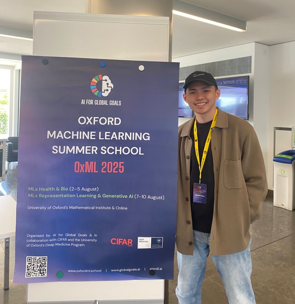
Just not long ago, I attended a machine learning summer school at University of Oxford's Mathematical Institute (Yes, THE Oxford)!
I guess I should start from the beginning.
Around two years ago, I started thinking about studying abroad to experience a different academic culture. Initially, I was curious about exchange programs, but I had some reservations. Living abroad for a semester seemed expensive, there was a chance it might delay my graduation, and I wasn't sure if my resume was strong enough for a scholarship.
So, I started looking into summer schools since they're usually just one- to two-week programs and are more affordable! I was particularly interested in a machine learning summer school. After doing some research, I found one happening at Oxford in August 2025! I didn't know what to expect, but I knew I wanted to give it a shot. So, I prepped my resume and applied without many expectations. About a month later (November 2024), I got a reply — and they offered me a place with a student discount!
I accepted without much hesitation because, let's be real, this is probably my only chance to set foot at THE Oxford University. And yes, it's going to be insanely expensive! I had to dip into most of my savings for this.
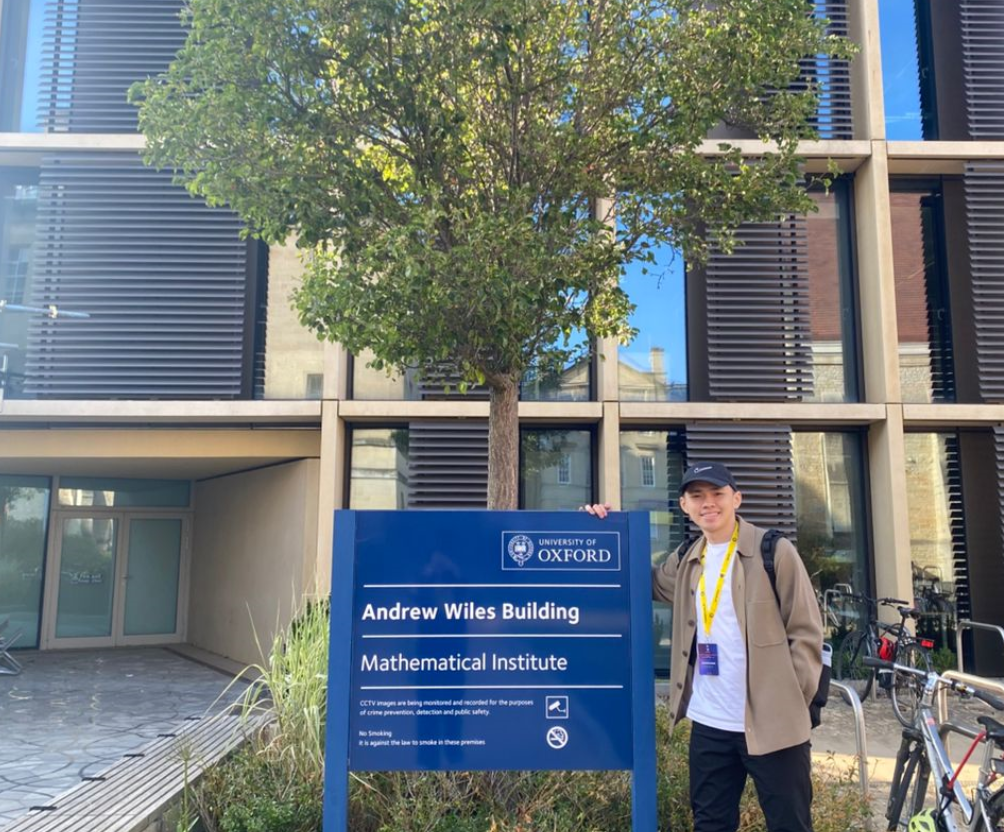
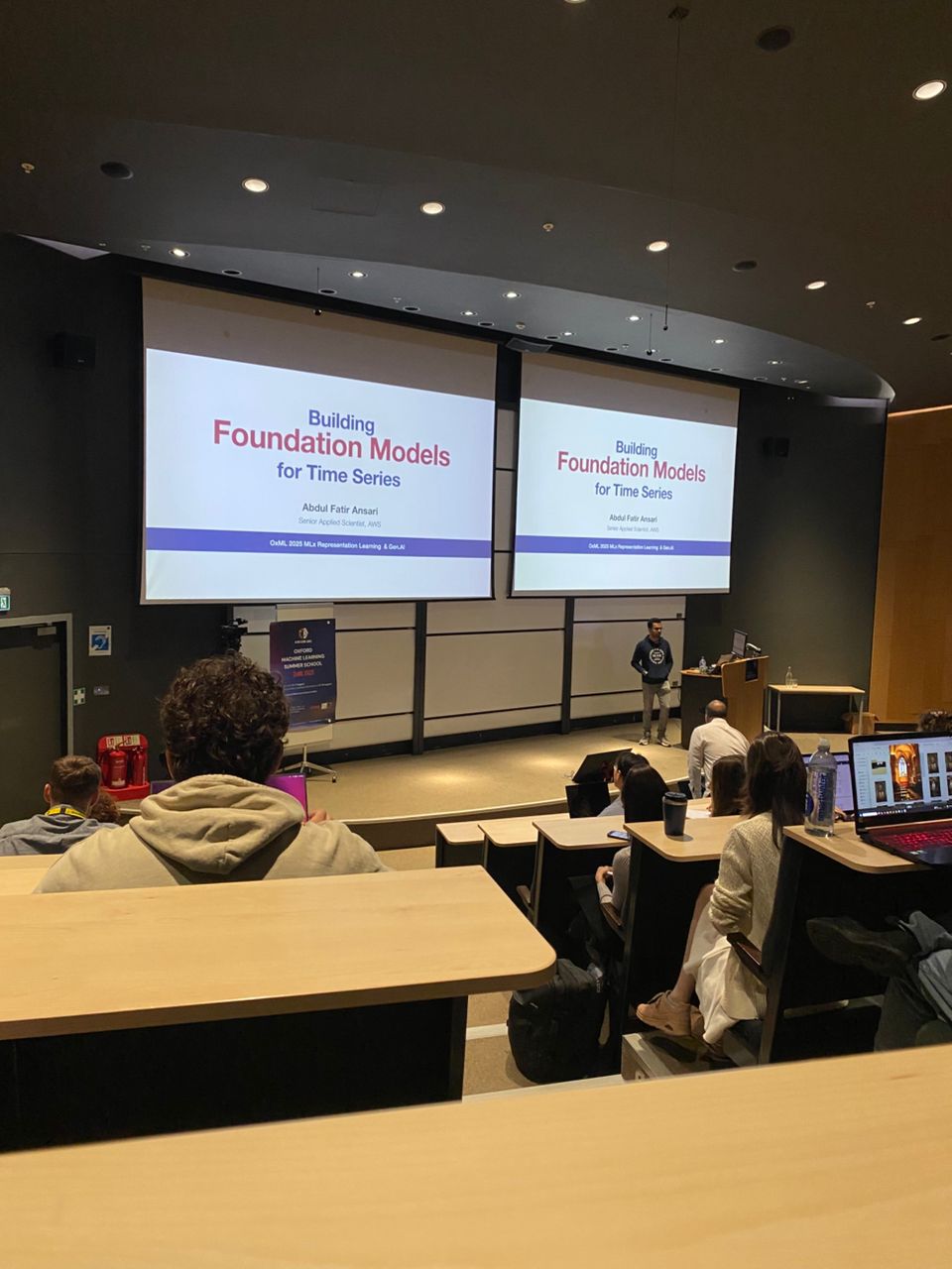
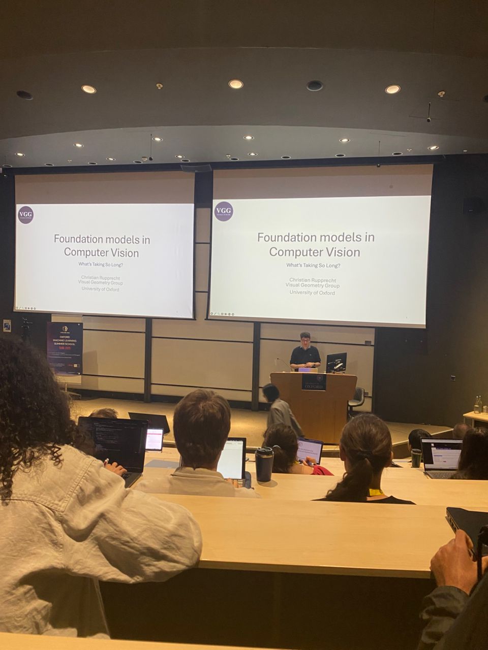
Fast forward to August 2025, and I made it to the Andrew Wiles Building at Oxford's Mathematical Institute!
When I arrived, I immediately felt like I didn't quite belong because almost everyone else was either a Master's or PhD student, and I was one of the few undergraduates there.
But honestly, that turned out to be a blessing. I got to learn so much from everyone around me, and the next four days were packed with fascinating talks by brilliant researchers from all over the world, plus some amazing opportunities to connect with people in academia globally!
Haha, no more yapping! Let's dive into OxML!
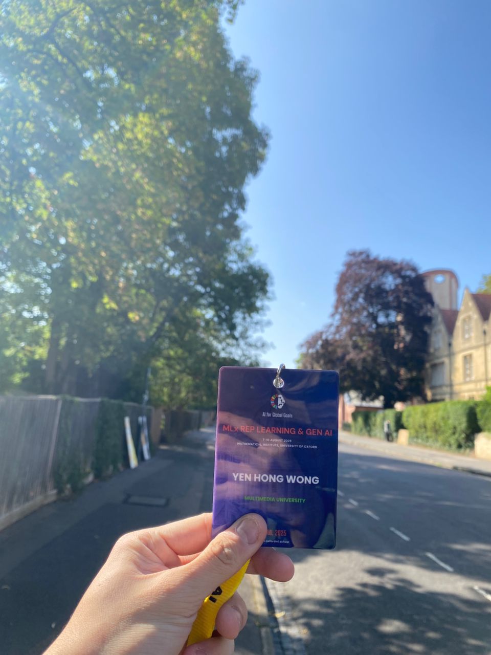
The track I joined was MLx Representation Learning & GenAI. If you don't know already, Representation Learning is about learning how to represent raw data in a way that captures important patterns or structures, one example being word embeddings. And GenAI? Well, who doesn’t know what it is nowadays?
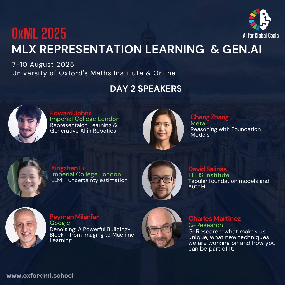
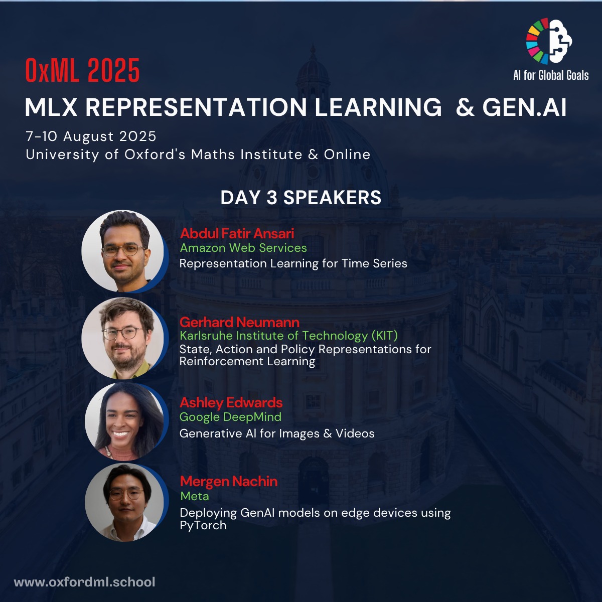
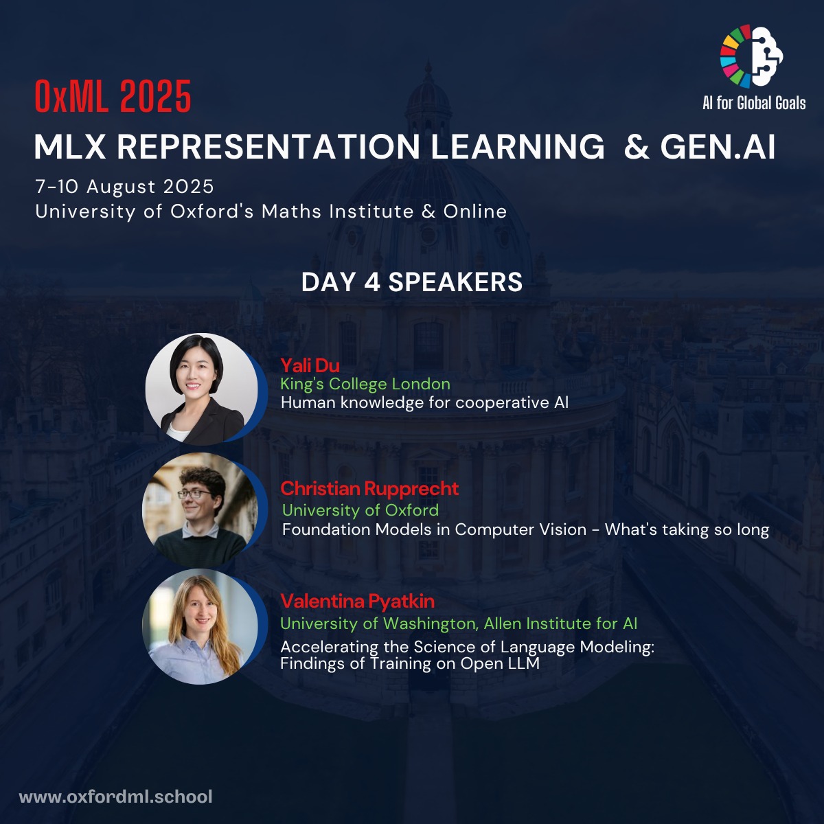
And here is the speaker line-up for this four-day program:
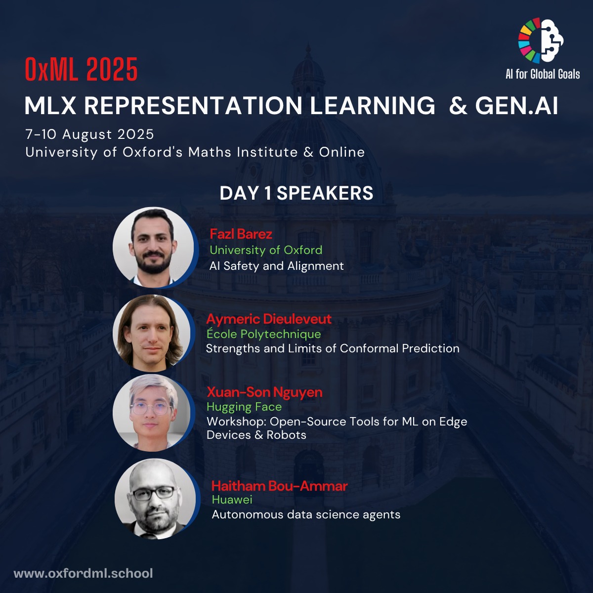
Some of the talks were super interesting, and I'd love to go through each one, but I honestly don't have the time (or the will) to lay them all out here. So instead, I'll just share the two biggest takeaways from OxML for me: Foundation Models and AI in Robotics.
Foundation Models
The content of this section is based on two talks: Representation Learning for Time Series by Abdul Fatir Ansari from AWS, and Foundation Models in CV by Christian Rupprecht from the Visual Geometry Group at Oxford.
You've probably heard a lot about Foundation Models lately, it's what everyone's talking about. But what exactly are Foundation Models?
The definition can be a bit fuzzy because people mean different things. If you do a quick Google search, most definitions look something like this:
A foundation model is a large-scale AI model trained on massive, diverse datasets that can be adapted to a wide range of tasks, serving as a base for more specialized applications.
The key characteristics are large-scale pretraining, general-purpose capability, adaptability, emergent behavior, and, in some cases, multimodality. Some examples that we're most familiar with are GPT and LLaMA. They are pretrained on huge datasets, can handle many tasks (summarizing, Q&A, etc.), can be adapted to specific domains with fine-tuning and sometimes surprise us with new abilities.
Although people emphasize different parts, most agree on those three core characteristics: large-scale pretraining, general-purpose, and adaptability. In OxML we looked at foundation models that meet these traits in areas like time-series forecasting and computer vision.
Chronos
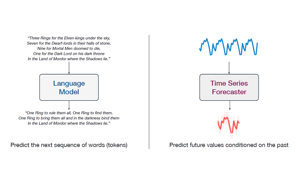
In language models like GPT, we're essentially performing next-token prediction. So, what if we could apply the same idea to time series data? Given the values at each point in the past, we could forecast future values, just like predicting the next word in a sentence. In language models, training on large-scale data leads to strong performance on previously unseen inputs. What if we could do the same for time series data, training a model that can generalize and forecast on time series it has never seen before?
And that's exactly what Chronos does! It frames the forecasting problem as a language modeling task. Like large language models, it also uses transformers!
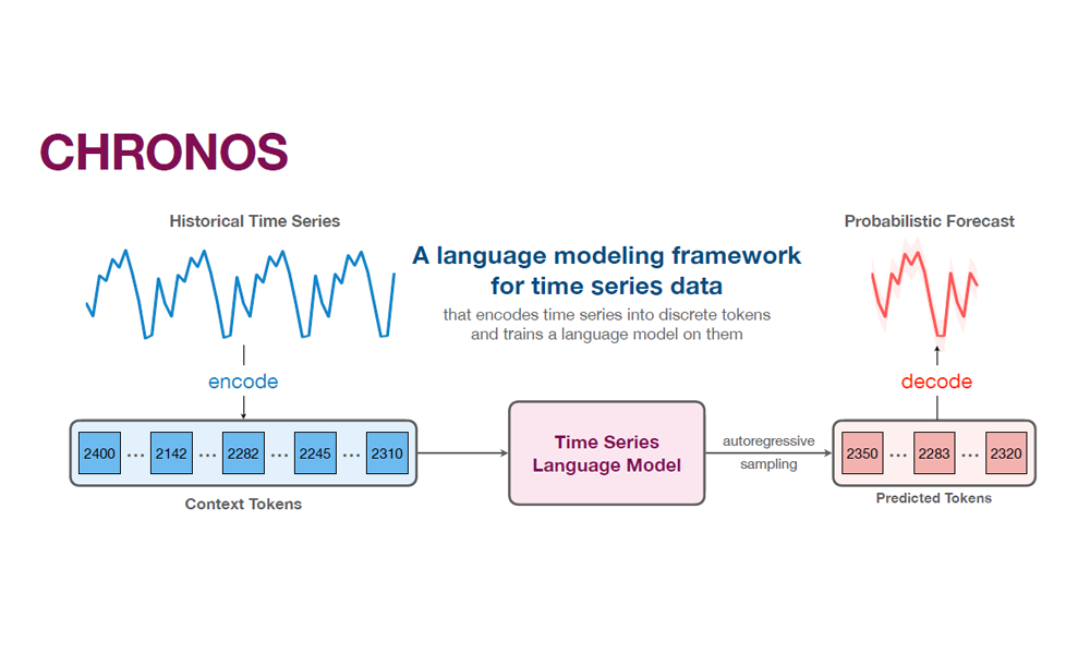
However, in order to model time series forecasting as a language problem, we first need to figure out how to feed the model input in time series like language. The difference between these two types of input is that word in language comes from discrete vocabulary, while time series values are real-valued.
To adapt them for a language-modeling approach, mean-scaling and quantization are used to discretize the values. This also means that forecasting becomes a classification task rather than a regression one. The upside of this is that it allows the model to output a distribution over possible future values.
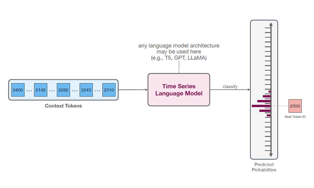
The design of this model is simple and intuitive, probabilistic by nature, and requires no changes to the language model architecture or training procedure.
To train a general-purpose time series forecasting model, a comprehensive collection of datasets from multiple domains was gathered. To address the limitations of small training datasets, two novel data augmentation techniques are proposed to enhance model robustness and generalization.
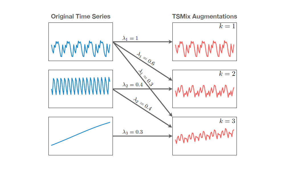
The first is TSMixUp augmentation, where we sample time series and a -dimensional weight vector from a Dirichlet distribution (a fancy term for vectors of positive values that sum to ). We then create a new time series by taking a weighted linear combination of the sampled time series.
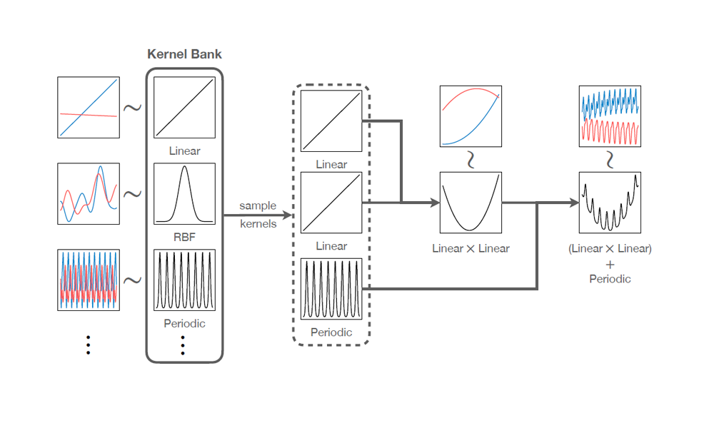
The second technique is KernelSynth, where kernels (i.e., patterns) sampled from a kernel bank are mixed with generic synthetic data to generate new, diverse time series.
Quantitative and qualitative results show that Chronos outperforms most task-specific models when used to predict previously unseen data and achieves state-of-the-art performance when fine-tuned on domain-specific datasets.
Several extensions have been developed based on Chronos, including a wavelet-based tokenizer, which replaces uniform quantization to better capture spikes in the data, Chronos-Bolt, a faster and more accurate variant of Chronos, and ChronosX, which enables the incorporation of exogenous variables, allowing for multivariate input.
Fun fact: I had the chance to work with the Chronos model at Grab just weeks before OxML, so getting to see the team behind this amazing work was truly special.
DINOv2
Chronos addresses the lack of a general-purpose model in time series forecasting. In the world of 2D computer vision, DINOv2 serves a similar role by providing a strong, general-purpose representation model.
Like Chronos, it's built entirely on transformers, specifically Vision Transformers. What makes it so powerful is its training approach. DINOv2 is trained in a self-supervised manner on a massive dataset of images, curated using a novel data processing pipeline that requires no human intervention.
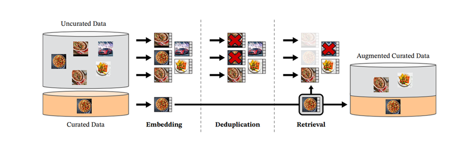
During data curation, this pipeline was implemented at scale using GPU-accelerated indices to efficiently perform nearest-embedding searches on a compute cluster of 20 nodes, each equipped with eight 32GB GPUs. In less than two days, a high-quality dataset called LVD-142M, consisting of 142 million images, was curated.
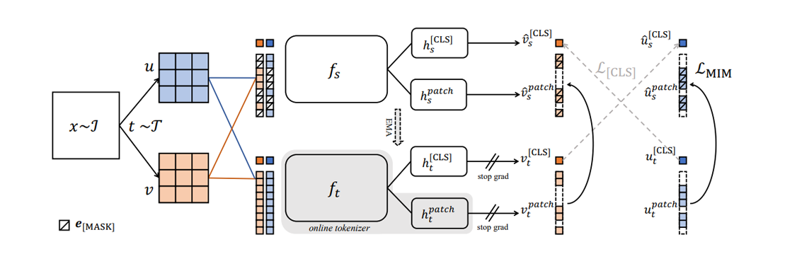
During training, DINOv2 uses both a student network and a teacher network, with the goal of learning image representations by supervising the student network's output using the teacher network's output. To achieve this, it optimizes two training objectives: an image-level objective from DINO (v1) and a patch-level objective from iBOT.
For the image-level objective, DINOv2 samples two different crops from an image and feeds them into the vision transformers of the student and teacher networks. The resulting class tokens are then passed to their respective DINO heads. The student's class token output is supervised against the teacher's class token output using a cross-entropy loss:
To ensure consistency and stable training, only the parameters of the student network are learned, while the parameters of the teacher network are maintained as an exponential moving average (EMA) of the student network.
For the patch-level objective, DINOv2 masks some of the input patches given to the student network but not to the teacher network, and passes them to both networks. The respective iBOT heads are then applied to the masked tokens for the student and the corresponding tokens for the teacher. Similarly, the student's tokens are supervised against the teacher's tokens using cross-entropy loss:
Here, is the index of the masked patch for the student. The parameters are trained in the same manner as in the image-level objective.
This entire process is similar to how it was done in iBOT:
DINOv2 was trained using the procedures described above, along with a few additional techniques. These include centering the teacher's output using Sinkhorn-Knopp centering, applying the KoLeo regularizer to encourage more even feature distribution across the space, and increasing the image resolution briefly at the end of training to improve performance on downstream pixel-level tasks.
DINOv2 can be adapted to a wide range of downstream tasks such as classification, segmentation, depth estimation, and zero-shot learning. It has demonstrated impressive results across all these tasks. Since its introduction, many papers have adopted DINOv2 as a backbone for their own downstream applications.
VGGT
DINOv2 performs very well, but only on 2D images. To address the 3D domain, the Visual Geometry Grounded Transformer (VGGT) is proposed. It reconstructs 3D scenes from multiple views by predicting a set of 3D attributes such as camera parameters, depth maps, point maps, and 3D point tracks in a single forward pass, unlike traditional methods.
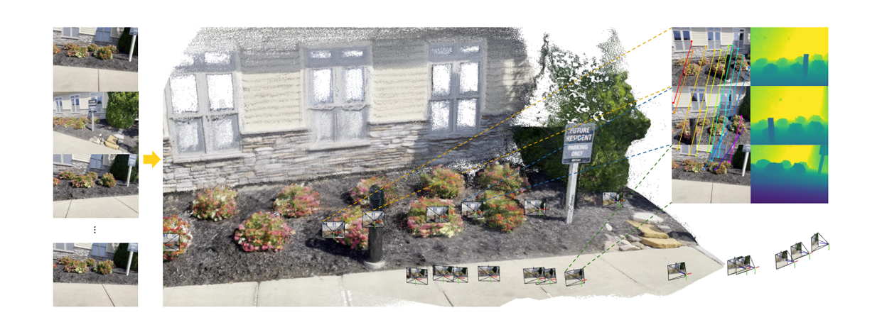
Although some of the quantities predicted by VGGT can be derived from one or more other attributes, for example, camera parameters can be inferred from the point map, it has been shown that explicitly predicting all attributes leads to performance gains.
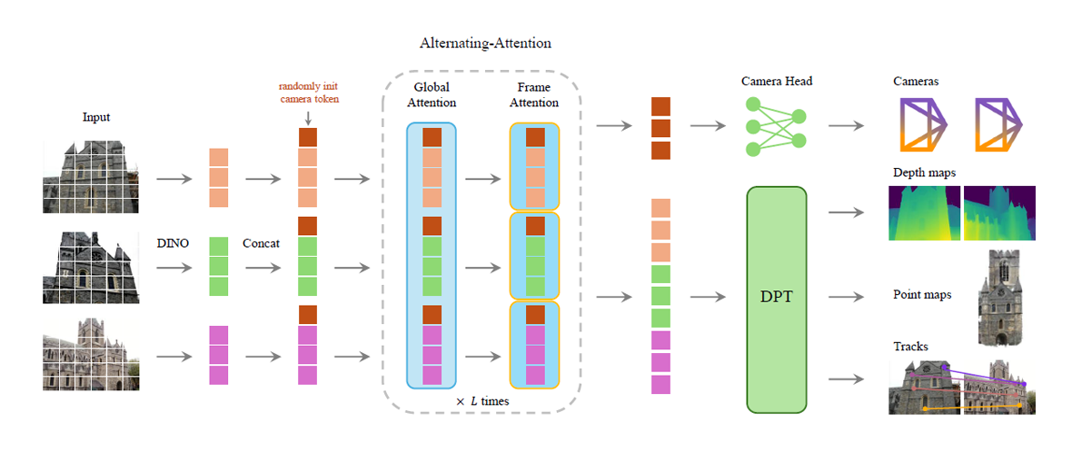
VGGT is, once again (you guessed it), a transformer! First, it passes all the frames through DINO (2D foundation model) to obtain the 2D representations. Then, a learnable camera token is prepended to the tokens obtained from DINO before passing them into the transformer.
VGGT also modifies the standard transformer architecture by introducing Alternating Attention (AA). Each iteration of AA consists of two stages: the first is global attention, which performs attention both within and across frames, and the second is frame attention, which performs attention only within each individual frame. The goal of global attention is to ensure scene-level coherence, while frame attention eliminates the need for frame positional embeddings, allowing frame permutation equivariance and flexible input length. Finally, the outputs are fed to the corresponding heads to predict the 3D attributes.
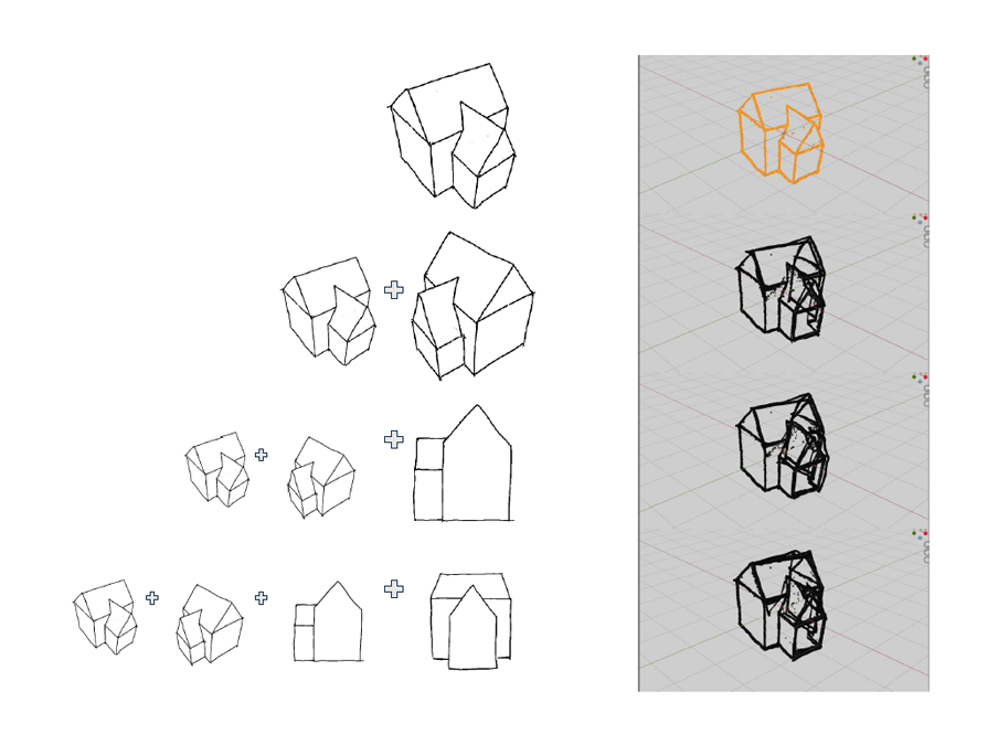
Qualitative and quantitative results have shown that VGGT achieves state-of-the-art performance and speed in multiple 3D tasks. Surprisingly, VGGT also learns to generalize beyond the training data and performs reasonably well on 3D reconstruction from concept sketches.
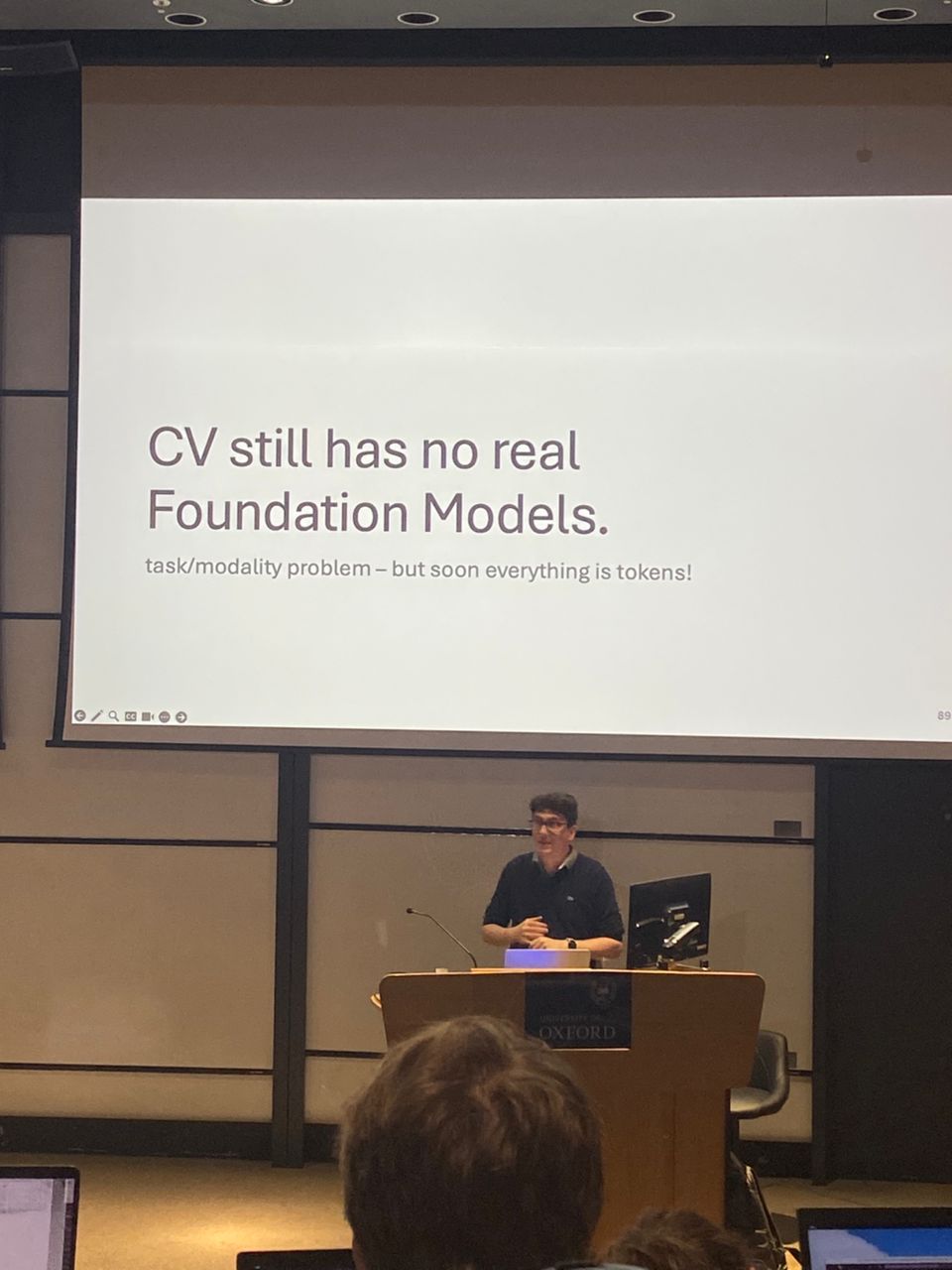
And that's all the foundation models I have for you. One of the speakers believe that we don't really have true foundation models in computer vision yet, because he has a strict definition of what a foundation model is. He believes that one key aspect all of these computer vision foundation models are missing is multimodality, since each modality (like 2D or 3D) currently requires a different model. But there was one interesting point he mentioned:
Soon, everything will be tokens. Everything is a transformer now. We're take images and turn them into tokens, we take 3D geometry and turn them into tokens. If everything is suddenly a token, maybe we can just train a model on all of these tokens and we don't have to deal with completely different modalities.
And yes, everything is secretly a transformer nowadays and maybe this is how we can finally achieve a true foundation model one day.
AI in Robotics
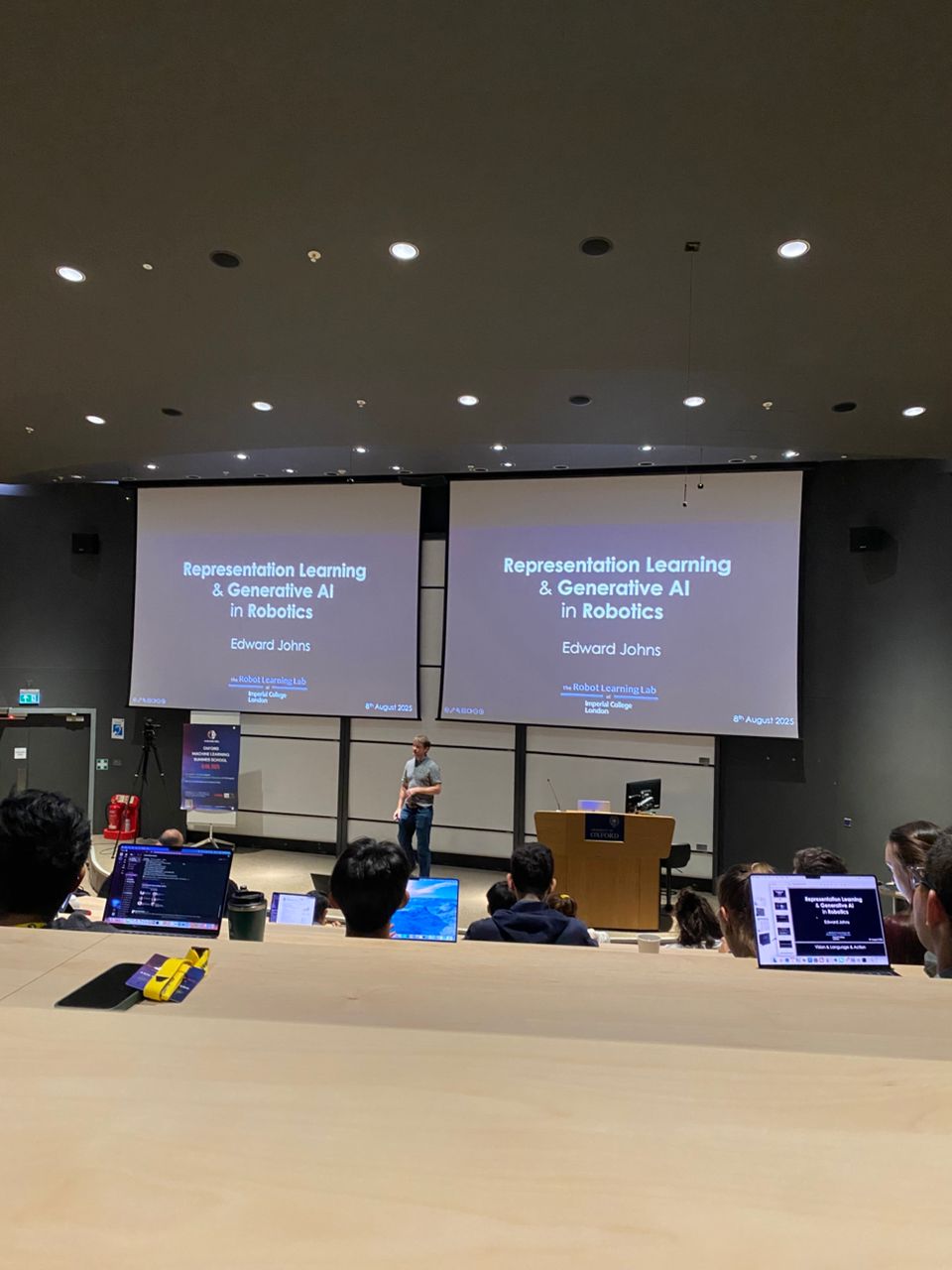
The content of this section is based on the talk: Representation Learning & Generative AI in Robotics by Edward Johns from The Robot Learning Lab at Imperial.
I've always thought AI in robotics was super cool. It's like the missing link that connects AI to the real world. But before this, I didn't know anything about the field because it's not really accessible where I'm from, and I had zero experience with robotics.
That changed when I joined OxML. I got to learn a ton about what's happening in the field right now through some really interesting talks on AI in robotics. Honestly, the future of this space looks both exciting and a little scary!
Anyway, I just wanted to share a few cool projects from the talks that really stood out to me.
Can Large Language Model Solve Robotics AI Task?
What if we could just prompt out-of-the-box LLM to solve robotics task?
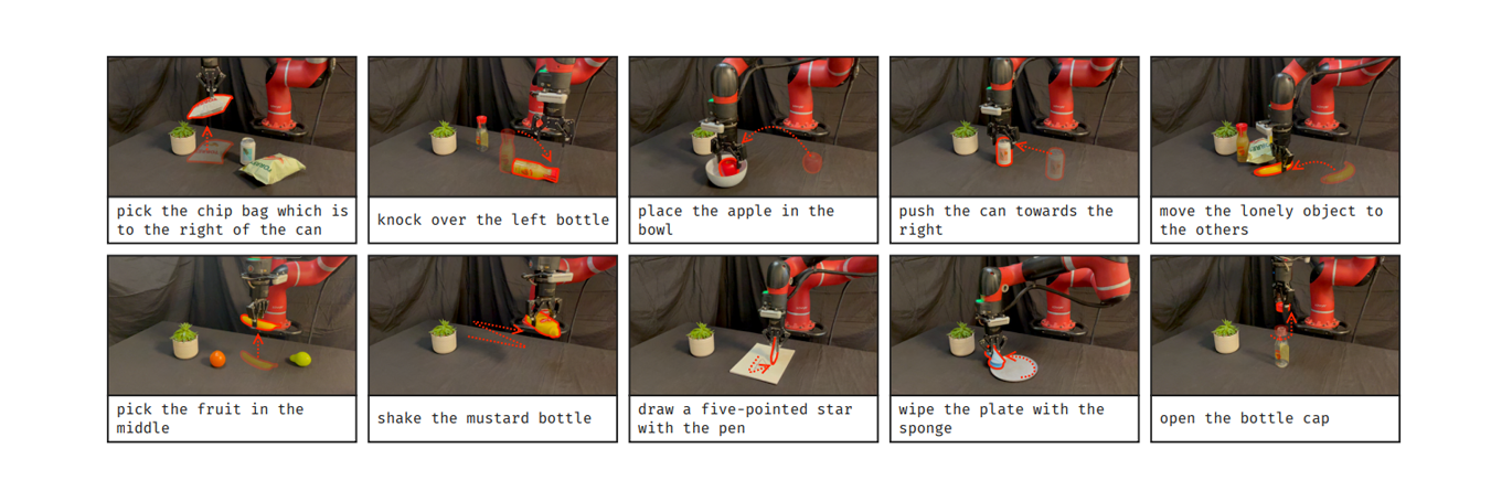
This work introduced a way to guide LLM to generate the sequence of actions for a robotics arm to complete manipulation tasks with a task-agnostic prompt and an object detection model. It shows that we can do this without the need for pre-trained skills, motion primitives, trajectory optimizers, or in-context examples, which are the techniques that have been used for previous methods.
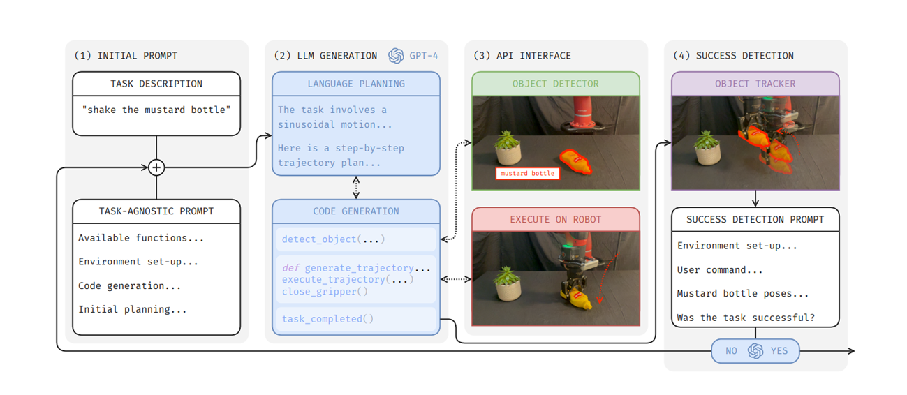
First, the user-provided task description (e.g., "shake the mustard bottle") is incorporated into a task-agnostic prompt and passed to the LLM. The LLM then performs high-level planning in natural language to determine how to complete the task. Based on this plan, it generates Python functions to interface with the object detection model and to execute the planned trajectories on the robot arm.
After the task is executed, a success detection prompt containing information about the state of the objects and environment is given to the LLM to assess whether the task was successful. If the attempt fails, the LLM is prompted to analyze what went wrong and retry the task with appropriate corrections.
Let's dive into the task-agnostic prompt because that's where the real magic happens. This prompt essentially gives the LLM all the information it needs to understand the task and figure out how to accomplish it. Some key components include:
- Available functions: A list of Python functions the LLM can call, such as
detect_objects(to interface with the object detection model) andexecute_trajectories(to execute planned movements using the robot arm). - Environment setup: Information about the current position of the robot arm and the mechanics or structure of the arm itself.
- Planning steps: Guidance on how to generate code and take actions based on the output of previous code snippets.
I’ve included the full prompt here if you'd like to take a look:
Full Prompt
# INPUT: [INSERT EE POSITION], [INSERT TASK]
MAIN_PROMPT = \
"""You are a sentient AI that can control a robot arm by generating Python code which outputs a list of trajectory points for the robot arm end-effector to follow to complete a given user command.
Each element in the trajectory list is an end-effector pose, and should be of length 4, comprising a 3D position and a rotation value.

AVAILABLE FUNCTIONS:
You must remember that this conversation is a monologue, and that you are in control. I am not able to assist you with any questions, and you must output the final code yourself by making use of the available information, common sense, and general knowledge.
You are, however, able to call any of the following Python functions, if required, as often as you want:
1. detect_object(object_or_object_part: str) -> None: This function will not return anything, but only print the position, orientation, and dimensions of any object or object part in the environment. This information will be printed for as many instances of the queried object or object part in the environment. If there are multiple objects or object parts to detect, call one function for each object or object part, all before executing any trajectories. The unit is in metres.
2. execute_trajectory(trajectory: list) -> None: This function will execute the list of trajectory points on the robot arm end-effector, and will also not return anything.
3. open_gripper() -> None: This function will open the gripper on the robot arm, and will also not return anything.
4. close_gripper() -> None: This function will close the gripper on the robot arm, and will also not return anything.
5. task_completed() -> None: Call this function only when the task has been completed. This function will also not return anything.
When calling any of the functions, make sure to stop generation after each function call and wait for it to be executed, before calling another function and continuing with your plan.

ENVIRONMENT SET-UP:
The 3D coordinate system of the environment is as follows:
    1. The x-axis is in the horizontal direction, increasing to the right.
    2. The y-axis is in the depth direction, increasing away from you.
    3. The z-axis is in the vertical direction, increasing upwards.
The robot arm end-effector is currently positioned at [INSERT EE POSITION], with the rotation value at 0, and the gripper open.
The robot arm is in a top-down set-up, with the end-effector facing down onto a tabletop. The end-effector is therefore able to rotate about the z-axis, from -pi to pi radians.
The end-effector gripper has two fingers, and they are currently parallel to the x-axis.
The gripper can only grasp objects along sides which are shorter than 0.08.
Negative rotation values represent clockwise rotation, and positive rotation values represent anticlockwise rotation. The rotation values should be in radians.

COLLISION AVOIDANCE:
If the task requires interaction with multiple objects:
1. Make sure to consider the object widths, lengths, and heights so that an object does not collide with another object or with the tabletop, unless necessary.
2. It may help to generate additional trajectories and add specific waypoints (calculated from the given object information) to clear objects and the tabletop and avoid collisions, if necessary.

VELOCITY CONTROL:
1. The default speed of the robot arm end-effector is 100 points per trajectory.
2. If you need to make the end-effector follow a particular trajectory more quickly, then generate fewer points for the trajectory, and vice versa.

CODE GENERATION:
When generating the code for the trajectory, do the following:
1. Describe briefly the shape of the motion trajectory required to complete the task.
2. The trajectory could be broken down into multiple steps. In that case, each trajectory step (at default speed) should contain at least 100 points. Define general functions which can be reused for the different trajectory steps whenever possible, but make sure to define new functions whenever a new motion is required. Output a step-by-step reasoning before generating the code.
3. If the trajectory is broken down into multiple steps, make sure to chain them such that the start point of trajectory_2 is the same as the end point of trajectory_1 and so on, to ensure a smooth overall trajectory. Call the execute_trajectory function after each trajectory step.
4. When defining the functions, specify the required parameters, and document them clearly in the code. Make sure to include the orientation parameter.
5. If you want to print the calculated value of a variable to use later, make sure to use the print function to three decimal places, instead of simply writing the variable name. Do not print any of the trajectory variables, since the output will be too long.
6. Mark any code clearly with the ```python and ``` tags.

INITIAL PLANNING 1:
If the task requires interaction with an object part (as opposed to the object as a whole), describe which part of the object would be most suitable for the gripper to interact with.
Then, detect the necessary objects in the environment. Stop generation after this step to wait until you obtain the printed outputs from the detect_object function calls.

INITIAL PLANNING 2:
Then, output Python code to decide which object to interact with, if there are multiple instances of the same object.
Then, describe how best to approach the object (for example, approaching the midpoint of the object, or one of its edges, etc.), depending on the nature of the task, or the object dimensions, etc.
Then, output a detailed step-by-step plan for the trajectory, including when to lower the gripper to make contact with the object, if necessary.
Finally, perform each of these steps one by one. Name each trajectory variable with the trajectory number.
Stop generation after each code block to wait for it to finish executing before continuing with your plan.

The user command is "[INSERT TASK]".
"""
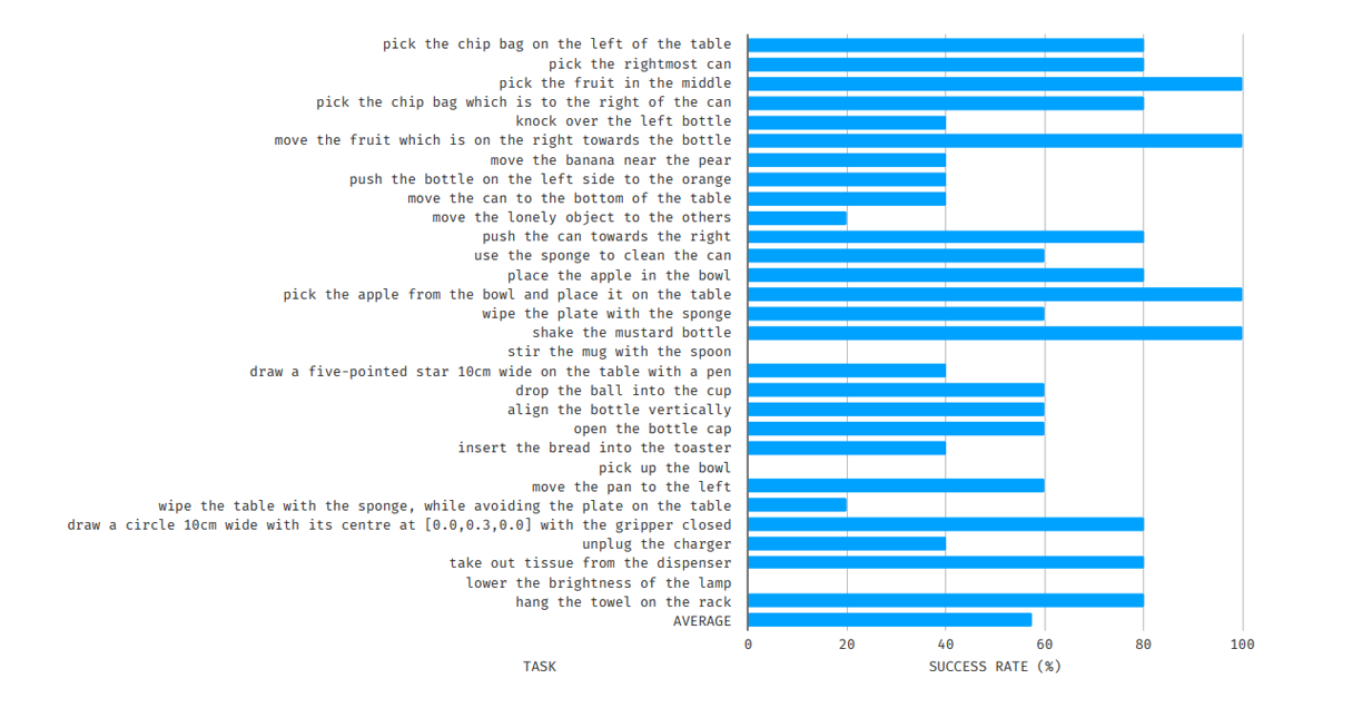
And it turns out this simple approach worked reasonably well on these day-to-day tasks!
Here's the success rate for the 30 day-to-day tasks. Not bad at all, especially considering it was done in zero-shot!
In-Context Imitation Learning via Instant Policy
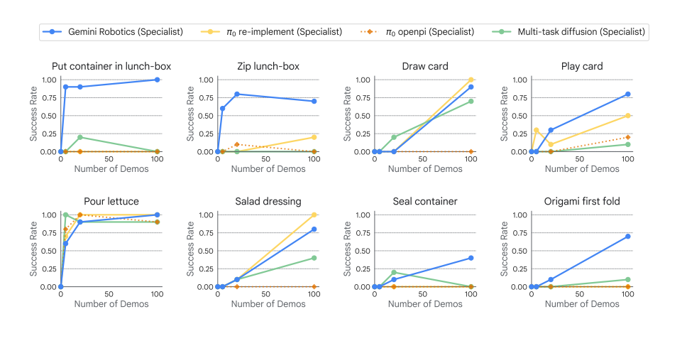
Traditionally, to teach a robot to perform a simple task, it could take thousand of hours to train a robot from pre-training to post-training before deploying to the real world. In fact, for Gemini Robotics, it takes almost 100 of demonstrations before the model reaches a high success rate:
While for human, we usually only need one demonstration to learn how to perform a simple task. And that's what Instant Policy (IP) is trying to address, by learning instantly from one demonstration or one-shot learning. IP does so by in-context learning. One great example of in-context learning is LLM, imagine you give LLM this prompt:
Complete the pattern:

(1, 1), (1, 2), (2, 2), (2, 1)
(1, 3), (1, 6), (4, 6), (4, 3)
(5, 1), (5, 3), (7, 3), (7, 1)
(6, 4), (6, 6), (8, 6),   ??
LLM will tell you it's (8, 4) and it does so by observing the previous examples. In a robotics task, it's similar. Given some demonostrations, each denoted by and the current observation , what is the action to take?
However, before we dive into the solution, let's first talk about two problems traditional approaches faced:
- They lacked inductive bias in observation and action representation. Most traditional approaches try to map images to action vectors, which can make it difficult for the model to generalize.
- They didn't have enough data to learn robust policies. There's a limited amount of real-world robotic datasets.
To tackle the first challenge, IP represents the observations and actions as nodes in a graph neural network:
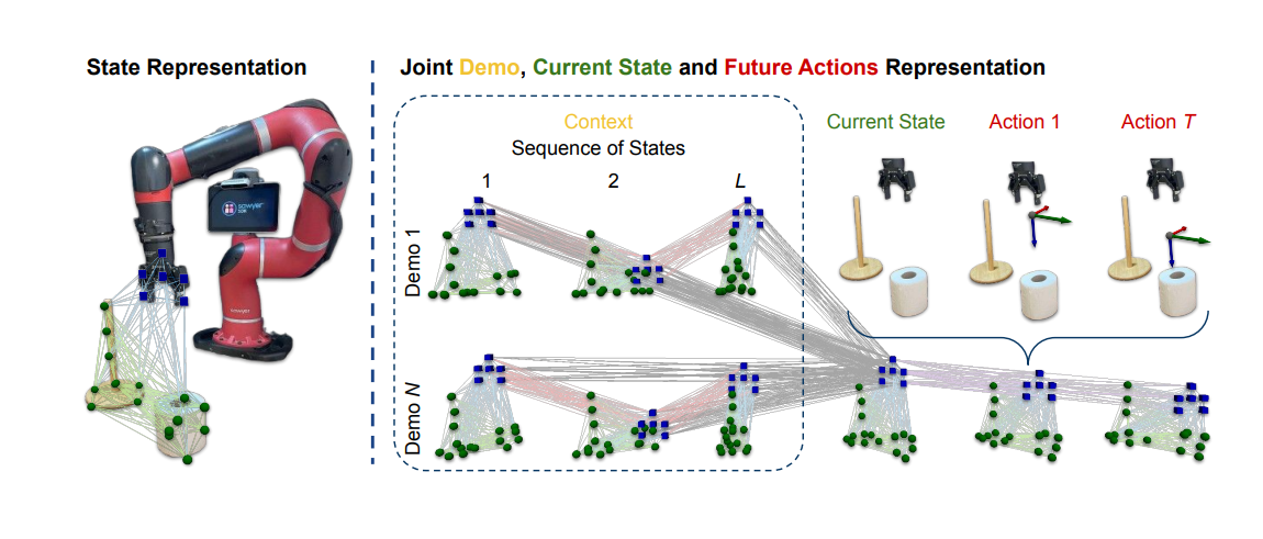
The flexibility of representing the information in a graph allows IP to incorporate any number of demonstrations and connect them to the current observation (the combination of demonstrations and the current observation is known as the context). Within each time frame, the nodes representing the objects and the grippers are connected via edges that encode the positional differences between them. Between each time frame in a demonstration, the gripper's nodes are connected to represent their relative movement. The gripper's nodes from the demonstrations are also connected to the gripper's nodes of the current observation to propagate relevant information. To express future actions, "imaginary" graphs are constructed in a similar manner, with the gripper's nodes connected across timesteps. This representation ensures that features can be aggregated and propagated in a meaningful and consistent manner. It addresses the first challenge because now our observation and action spaces are aligned — they have the same modality, just nodes in a graph.
The next interesting part of this method is how it predicts actions through graph diffusion.
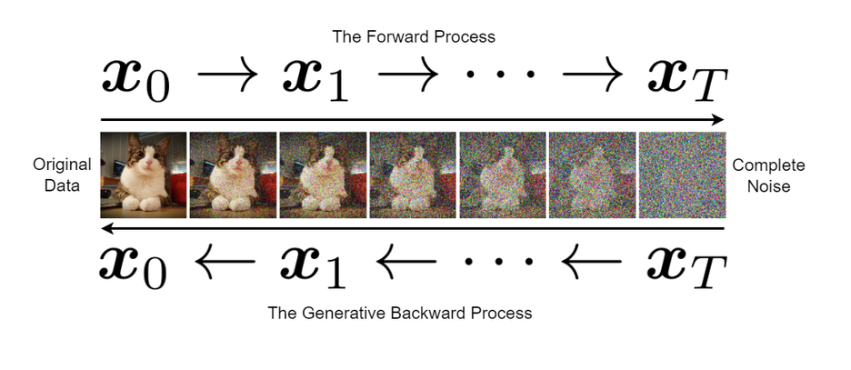
Personally, I don't know much about diffusion, but here's the gist of it: we train a model to denoise random white noise sampled from a normal distribution, which enables us to generate something random from it. There are two processes in diffusion. The forward process starts with a clean example from the dataset and progressively adds white noise until it becomes random white noise in steps. The backward process takes the white noise and gradually refines it to resemble a clean data sample by denoising it step by step. A model is trained to predict the added noise at each step of the forward process, enabling it to reverse the process and generate clean data from pure noise.
Graph diffusion is essentially diffusion applied to a graph. The goal is to encode future actions into a normal distribution, from which we can sample. In IP, a graph transformer is used for denoising, enabling the generation of valid actions for a given graph input. By using diffusion instead of direct prediction, the model can capture the complex distribution of actions, predicting them gradually rather than making a direct prediction all at once. This approach enhances the model's ability to handle uncertainty and produce more diverse and realistic actions.
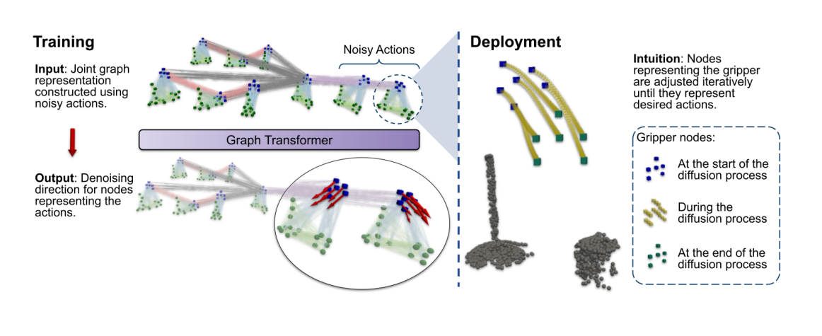
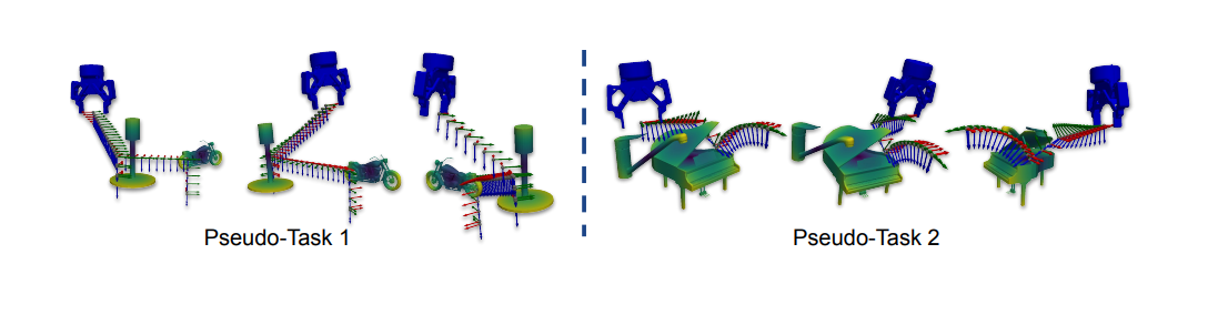
The graph diffusion process, visualized for multiple future actions:
Now, the second challenge — lack of data. Because in-context learning is used, the model doesn't need to learn a specific task during pre-training. This means we can train the model with simulated data that is "arbitrary but consistent," meaning that these simulations are essentially the same type of pseudo-task at a semantic level. This approach essentially allows us to pre-train the model with an infinite pool of simulations.
As a result, with instant-policy, the robot only needs one demonstration:
Both quantitative and qualitative results show that the robot's instant-policy performs strongly compared to the baselines.
Overall, I learned a lot from OxML.
Was it worth it? YES, even though it was pretty expensive. But, I made sure to make the most of it — explored plenty of fascinating placess across the UK. Read how that went.