I originally planned to write about some of the topics I had learned in OxML and include all of them in my OxML blog. Conformal Prediction was the first and so far, the only one I have completed. After some time, I realized that finishing it entirely would take far too long, especially with how busy life has been. So, I decided to let go of this idea for now. Still, I didn't want this write up to go to waste. So, here it is.

Strengths and Limitations of Conformal Prediction by Aymeric Dieuleveut at OxML 2025.

Conformal prediction is a tool for quantifying uncertainty in model's prediction. Quantifying uncertainty is especially important in fields such as weather, medical, markets and, LLMs where a faulty model's prediction can have serious impacts to the consumers.

To understand what uncertainty is, imagine training a linear regression model on three different datasets, each having greater variance than the one before.

Linear Regression Model fitted on 3 different datasets.

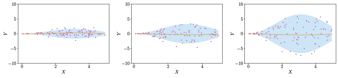
Notice all three datasets look very different from one another. However, the linear regression model seems to have fitted in the exact same way! Clearly, the quality of the model's fit varies across datasets but how do we express them? This is where quantifying uncertainty comes into play.

To put simply, the goal of conformal prediction is to construct a prediction set $C_\alpha$ given $X_{n+1}$ such that the probability of $Y_{n+1}$ falling within $C_\alpha(X_{n+1})$ is $1-\alpha$ while remaining agnostic to both the model and the data distribution. Formally, it is defined as follows:

PS: One can think of $C_\alpha$ as the confidence interval we learned about in basic statistics!

In this talk, we were introduced to the simplest form of conformal prediction, Split Conformal Prediction. Let's jump right in!

For simplicity, we focus only on the regression case. The idea of classification case is almost the same, you can look it up if you're interested. The procedure is as follows:

1. We split the training data, $(X_i, Y_i)^n_{i=1}$ into a training set and a calibration set.
2. We train a mean predictor, $\hat{\mu}$ on the training set.
3. We obtain the set of conformity scores $S$ using the mean predictor and the calibration set, defined as follows:

4. Compute the quantile score of the conformity scores $S$ at $1-\alpha$, denoted by $q_{1-\alpha}(S)$.
5. To quantify the uncertainty for $X_{n+1}$, compute $C_\alpha$ as follows:

The prediction set $C_\alpha$ for all possible points $X_{n+1}$ can be visualized as follows:

The blue region indicates the prediction set.

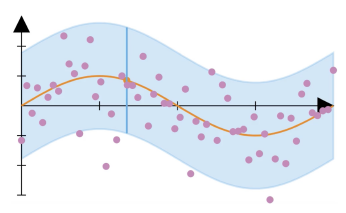
And that's it! The idea is quite intuitive. Essentially, we find the $1-\alpha$ quantile from the set of errors, denoted $q_{1-\alpha}$ and (under certain conditions) it can be guaranteed that, on average, the probability of an error exceeding $q_{1-\alpha}$ is $\alpha$!

The guarantee requires some assumptions about the dataset. In particular, the dataset $(X_i, Y_i)^n_{i=1}$ needs to be exchangeable, meaning that the joint distribution is the same as the joint distribution of any permutation of the original random variables. Exchangeability is ensured when the samples are i.i.d (independent and identically distributed). Under these assumptions, the theoretical guarantee holds, which can be proven using the quantile lemma. Again, you can look it up if you're interested! (Forgive my laziness!)

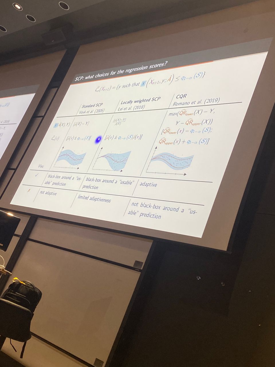
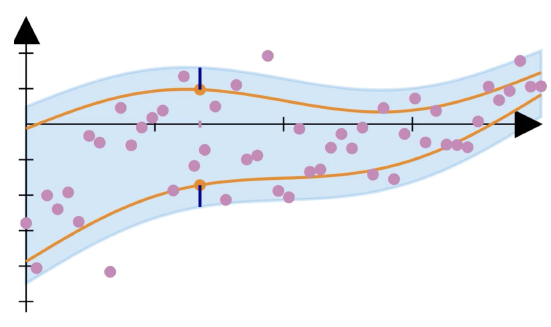
However, this method has some flaws. If you look at the previous diagram, you will notice that the size of the prediction set $|C_\alpha(X_{n+1})|$ is constant regardless of the properties of the data at a point. This is because when we use a mean predictor $\hat\mu$, we have no adaptability, since the mean for the dataset is fixed. To incorporate more adaptability, we can use a quantile regressor, $\hat{QR}$ instead. The procedure is very similar, with a few differences:

1. Definition for computing $S_i$:

2. Definition for computing $C_\alpha$:

As a result, we achieve greater adaptability, and the size of the prediction set $|C_\alpha(X_{n+1})|$ is no longer constant.

The blue region indicates the set.

To summarize, Split Conformal Prediction (SCP) is a simple, model-agnostic method for quantifying uncertainty that comes with theoretical guarantees, as long as the assumptions (exchangeable data) are met. However, it is not perfect. First, there is a data splitting issue: when we split our data, we trade off between the model quality and the calibration quality, which is not ideal. Methods such as full conformal prediction does not require data splitting, but they come at a cost to computational efficiency. Second, the thereotical guarantees are only marginal, not conditional: they ensure that prediction intervals contain the true value on average, not for each individual $x$. Third, exchangeability does not hold in many practical applications because data shifts in the real world (e.g., covariate shift and label shift).